Geometric generalization of map data and its importance for well readable maps is something I have written about quite a bit before. One of the main reasons why this subject is widely neglegted in practical map rendering is that plain color rendering has become the most common way to depict areas in maps in many cases. When using plain color rendering the need for geometric generalization is often much less obvious and less severe than with outlined or otherwise more sophisticated depictions. This essay will try to shed some light on the background and technical context of this. It offers practical ideas how to efficiently render these kinds of maps but I also hope to show how some current trends in map rendering are quite inconsistent.

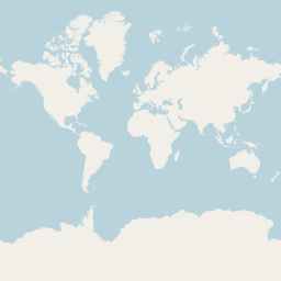
The iconic example of plain color area rendering in maps is the OpenStreetMap standard style at zoom level 0:

This also well serves as an example why this kind of rendering is so popular with web maps: It is extremely compact and efficient in terms of geometry representation in very small space. 256×256 pixel is really not a lot of room to represent information, yet the coastline in its shape is quite recognizable even at this scale. If you compare this to my generalized coastline rendering drawn with an outline at zoom 1

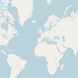
you see that while it certainly is clearer and cleaner in representation it accomplishes this by showing significantly less detail even at one zoom level higher. This removal of information is always a highly subjective choice. The apparently higher degree of objectivity is to a large extent what makes the non-generalized plain color rendering appealing to many people.

The other reason is the apparent lack of need for explicit generalization. This means you can usually generate this kind of rendering directly from the raw data without obvious flaws and problems as you would see when you try to do this with a drawn outline.

This is however often a serious misjudgment. The z0 coastline rendering above is close to being perfect but in other situations, especially with many small features, there are often significant errors.

The (almost universal) flaw of plain color area renderings

The most fundamental error comes from the way this kind of rendering is usually produced. In the simplest case - as demonstrated by the OSM coastline example - you have two colors and a polygon with the inside to be represented by one color and the outside by the other. The aim of plain color rendering is that every pixel in the rendering is colored with a mixture of the two colors depending on which fraction of the pixel is inside and which is outside the polygons shown.

In reality the color mixing is not linear due to gamma correction but it is a monotoneous function of the pixel coverage fraction.

So far the theory. In reality rendering is usually accurate as far as geometrically calculating the pixel coverage is concerned but is fundamentally flawed since it treats all polygons covering a pixel independently. You can easily imagine when rendering the zoom level 0 coastline most pixels near the coast contain a significant number of different polygons because for example several islands cover parts of the same pixel. So lets look at a simple example of a pixel with one quater covered by one polygon and another quater by another - the rest being uncovered. The rendering engines should obviously render this as a half covered pixel and mix the color accordingly.

What actually happens is that first they draw one of the polygons leading to a coverage of 25 percent (f₁=0.25) and then drawing the other mixing the additional 25 percent coverage (f₂=0.25) with the original one leading to

f_total = f₂ + (1-f₂)*f₁ = 0.25 + 0.75*0.25 = 0.4375

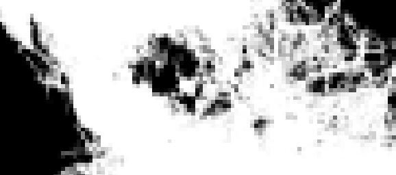
You can usually see this problem most clearly at the edges between adjacent polygons of the same color where some pixels have partial coverage by two polygons while areas around contain pixels covered fully by a single polygon and even though there is not actually a gap between the geometries in these pixels the background color shines through.

Typical rendering artefacts at edges of touching polygons

In reality this is further complicated by the mentioned need for gamma correction and a common technique to mitigate this issue is to manipulate or abuse the gamma correction to reduce artefacts because of this at the cost of overall rendering quality.

With small grained data the error in rendering might not be as obvious as in the examples shown but it still distorts the rendering results, sometimes quite significantly.

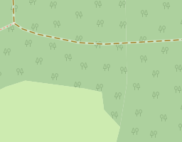
Polygon rendering artefacts and color distortions in the OSM standard style at z8

Dealing with lots of data

As mentioned plain color rendering is generally robust concerning the lack of geometric generalization, but in addition to the described basic flaw it is also fairly slow when you are dealing with lots of data. If you have a hundred different polygons intersecting a certain pixel - a scenario that is not unrealistic when you are rendering the low zoom levels based on very detailed data like in OSM - this takes a lot of time.

The usual methods to tackle this are filtering out small geometries and applying line simplifications to the polygon outlines. At first sight you might think that not considering all polygons with an area smaller than something like 1/256 of a pixel is safe to do without affecting the results but this is wrong of course because the accumulated size of these small areas can still be significant. At zoom 3 for example a pixel is 380 square kilometers in size. The OSM standard style filters with a one percent of the pixel area threshold. If you have within that pixel 20 lakes with an average size of two square kilometers and smaller than 3.8 square kilometers that would already be more than ten percent of the pixel area - and this is not an unrealistic scenario in reality.

Line simplification of the polygon outlines comes with the same problems essentially, errors tend to accumulate since small polygons are on average reduced in size by applying line simplification.

Both area filtering and line simplification are often applied rather aggressively by many map providers in the interest of cost reduction and higher throughput so that ultimately the artefacts generated by this sometimes exceed those due to the basic error of multiple polygon handling in the rendering engines.

Better ways

One fairly straight away solution to all of these problems is actually a very old technique. It is called supersampling. Instead of rendering the geometries by meticulously calculating intersections between them and the pixels you only test if the pixel center is inside or outside the geometries - but you do it at a much higher resolution. Kind of the brute force approach to rendering. The common wisdom taught in computer graphics is usually that this is very expensive to do and should be avoided where possible. But it depends on the circumstances of course and it is generally a good idea not to base decisions on dogmatically sticking to this kind of rule.

In web map rendering the fact that we are usually rendering a whole set of maps at different resolutions makes the supersampling approach very attractive in principle but taking advantage of this would mean breaking with the concept that map tiles are the basic atomic units of the rendering process that are rendered completely independently from each other.

The other reason why this approach has not gained any significant foothold in map rendering is that most map rendering frameworks are strongly tied to a forward rendering approach and have no good way of dealing with sampled data outside the scope of the final rendering grid.

Making use of supersampling for the purpose of plain color polygon rendering essentially means you sample the polygon data in a fine enough grid once (or in other words: rasterize it) and generate all renderings for the different zoom levels from this set of samples.

Data size considerations

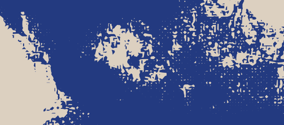
Using the OSM standard style z0 rendering as an example again - we would for a really good quality use a 16×16 supersampling and initially rasterize the coastline polygons data in a 4096×4096 points grid. The pixel coverage fractions of the data can then be determined from the primary sample grid by counting samples within the area of each pixel in the final 256×256 pixel image.

The pixel coverage fraction is calculated by counting the water samples (white) in the 16×16 samples within each pixel

In this simple form the only gain we have over the normal rendering approach is avoiding the multiple polygons rendering error as described above. Since we render only a single zoom level in this example there are no synergy effects from reusing the sample data in multiple renderings but you can easily imagine we can do the same for z1 with a 8192×8192 points grid (or be satisfied with 8×8 supersampling) and then get the z0 rendering essentially for free except for some additional sample counting.

What is also interesting is to look at the data volumes involved. The polygon data set normally used for rendering this is a 30MB shapefile that zips to a bit more than 20MB. As described above you can reduce that but this is generally a lossy process regarding rendering so the rendering results would differ.

The calculated pixel coverages - no matter if generated using classical rendering or with a supersampling approach - is, encoded with one Byte per pixel, 64kB in uncompressed form that compresses to a bit more than 10kB as PNG. And this is about as compact as you can get. No vector representation that renders into something even just broadly similar will likely get anywhere near this.

When we are talking about rendering vector data is only an efficient form of representation of information if the data density is small compared to the complexity and resolution of the chosen rendering. This is obviously the case when we are talking about things like POIs with icons, labels or even most line features but for plain color polygon rendering the size advantage always goes to a raster representation when the geometry is more detailed.

This is something that should probably be kept in mind by everyone who is following the vector tiles hype these days.

For comparison: the full original sample set with 16×16 samples per pixel is 2MB uncompressed or about 100kB compressed.

Selling wine in plastic bags

I have no illusions that directly rendering maps from sampled representations will be widely adopted any time soon. And as already indicated there are also many parts of map rendering where this is no advantage so it will never be able to compete with the classical rendering frameworks we have now as a one size fits all solution. And something like a more flexible hybrid rendering system that does not promise to kill all birds with one stone is not really in sight at the moment - at least not in the domain of map rendering.

What you can do in most rendering frameworks is using the aggregated fractional pixel coverages in raster form as a raster image source. You need to produce this externally for every map resolution (i.e. every zoom level) you need and in most cases you will be fairly limited in terms of styling options.

But even in a purely forward vector rendering based framework you can still make use of the advantages of supersampled rendering. The idea is to construct a vector data set from a supersampled grid that - when rendered using the usual rendering engines - approximately produces the results of a supersampled render.

So the task is to create a polygon data set that satisfies the following conditions

• when rendered it should produce a result as close as possible to a supersampling based rendering of the original geometries.
• it should be as small in data volume as possible so it does not take long to render and is compact in storage and transfer.

You might want to add a third requirement, namely that the data set should look reasonable when rendered at a higher resolution than the target resolution as well - or in other words: that it looks good in overzoomed rendering. This however quite strongly conflicts with the second goal so I only gave this minor consideration here.

Even the two main goals described are conflicting of course so in the end this is an exercise in compromise between the different goals. How this can look like can be seen in the following. It makes sense of course to align the sampling grid with the target rendering grid since to accomplish the first goal you will design the polygons so that each pixel in the taget rendering grid is covered by no more than one polygon and to a fraction that matches that of the supersampling data.

Pixel coverage fractions calculated with supersampling

Generated polygons representing the pixel coverage fractions

The most striking property of this synthetically generated polygon data set is probably that it does not necessarily bear any resemblence topologically with the original data. But keep in mind that for rendering at the target resolution this is not of any disadvantage. Both in appearance and in the underlying concept there is some similarity of this to halftoning patterns. The major difference is that halftoning patterns are physically printed while this vector data set is generated for purely virtual use.

You are not wrong if you think this approach is kind of weird because you generate a vector data set from a sampled grid representation just for the purpose of using it then to produce a raster rendering again. The only reason to do this is because many map rendering frameworks do not offer any other option - at least not without severe constraints in terms of styling or by doing all the rendering externally and just compositioning the rendered images.

How does it taste?

All the following samples use the proposed three class water coloring scheme.

First a direct comparison of conventional rendering based on the normal simplified water polygons and the vector representation discussed here.

Conventionally rendered coastline	Rendered using synthetically generated halftoning polygons

The two renderings are not exactly identical but relatively close with the difference being hardly visible without magnifying. The maximum error can be adjusted - this is ultimately a tradeoff between data set size and accuracy. And considering the mentioned errors and artefacts that occur with the conventional rendering approach we are in an area here where the differences in most cases are to similar parts due to errors in both versions or in other words: the truth probably lies in the middle.

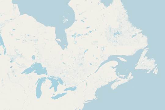
The really interesting part of course comes when we also render inland water areas. Here a set of example for zoom levels 0 to 5.

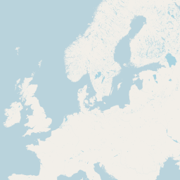
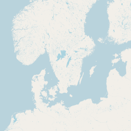
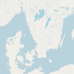
Rendering of ocean and inland water areas using vector representation

As a reminder: For z5 we are rendering all the surface water data from OSM here with a data volume of more than 6GB from a polygon data set of just about 120MB is shapefile format - with almost exactly the same rendering results.

The real thing

What i have shown above is based on the generated halftoning polygon representation. This can be used just like a normal polygon data set. You should not try to render it with outlines but in terms of area fills everything that can be done with polygons like fill patterns, color gradients etc. can also be used here in the same way.

But as already indicated above from a technical standpoint this is kind of weird so we can also forego the halftoning step and use the fractional pixel coverage raster data directly. This leads to severe styling limitations in most rendering engines but with plain color fills at least Mapnik can be persuaded to produce something similar:

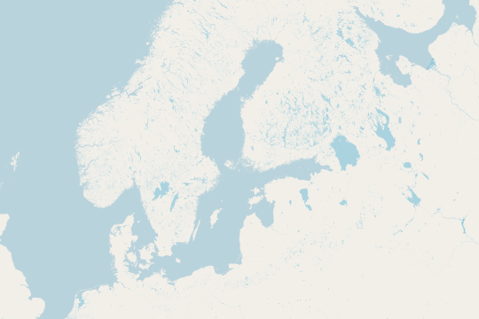
Rendering of ocean and inland water areas using supersampled raster data source

The big advantage of this approach is that the data volume is just a few percent of the vector version. For z5 instead of the 120MB of shapefiles we just have about 4MB as compressed TIFFs - again with almost exactly the same rendering results.

And where you can get it or brew it yourself

Preliminary experimental polygon sets for oceans, lakes and river areas in Mercator at z0-z6 can be found on:

ocean-polygons-reduced-3857.zip
lakes-polygons-reduced-3857.zip
river-polygons-reduced-3857.zip

Raster data sets with the fractional pixel coverages for the same are here:

ocean-raster-reduced-3857.zip
lakes-raster-reduced-3857.zip
river-raster-reduced-3857.zip

If you want to try out generating the polygon representations yourself you can find the halftoning tools on:

https://github.com/imagico/gray2vec

Christoph Hormann, November 2016