imagico.de

Earth render techniques demonstration scene

I have been asked a lot of times for sample code demonstrating the techniques of my earth renders in a practical example. While i don't mind giving such an example i am somewhat reluctant to dump some uncommented scene without actually explaining how things work. Here is my attempt to solve this.

This scene is licensed under the Creative Commons Attribution-ShareAlike 2.5 License.

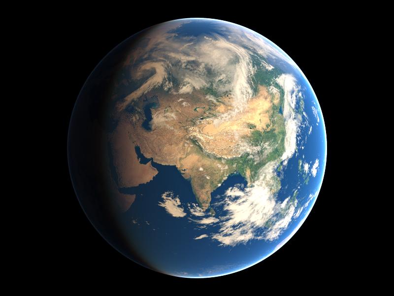
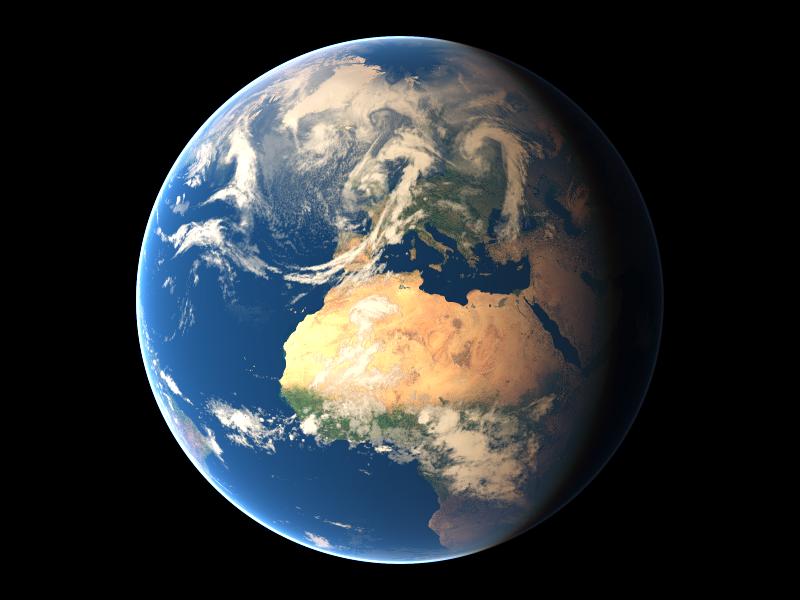
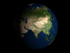
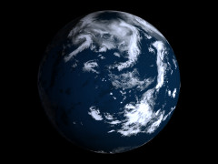
Below you can find the different sections of the scene explained. Get the full scene file to render it. There are three predefined camera and lighting setups which generate the views below:


view 1: Asia	view 2: Europe and Africa	view 3: North America

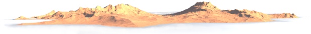
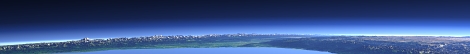
For small scale renders like the ones above the scene is in fact not well balanced. The expenses for the surface geometry are exaggerated compared to the fairly crude clouds. The use of an isosurface demonstrates the technique used in the other earth renders as a very efficient way to accurately render a detailed spherical surface based on elevation data files.

The scene settings

The scene begins with a number of variable definitions that set certain values for the scene to adjust lighting, atmosphere etc. The scale of the scene is 1 unit = 1 km.

// ========== advanced settings ===========

#declare Earth_Radius=6371;
#declare Height_Exaggerate=1;
#declare Terrain_Ambient=0.03;
#declare Terrain_Brightness=1.25;
#declare Max_Mountain=9;

#declare Media_Intensity=0.15;
#declare Media_Emission=0.065;
#declare Media_Eccentricity=0.56;
#declare Atmosphere_Top=100;

#declare Cloud_Brightness=0.42;
#declare Light_Intensity=4.1;

You can define which data files should be used for the surface geometry, coloring and clouds. The data used for the renders above is the ETOPO2 data set for the topography, the Blue Marble NG 2km July image for the coloring and a xplanet real time cloud map for the clouds. Note these data sets are quite large, rendering takes more than 800 MB of memory. For a small scale render you can use lower resolution data sources as well.

Since there have been occasional questions on how converting the ETOPO2 data set to a format readable by POV-Ray - this can be done using the ImageMagick conversion tools. Alternatively you can use any global elevation data set that is available in a format readable by POV-Ray, for example using a WMS version of the SRTM30 set. Obtaining a high resolution global image this way requires you to assemble it from tiles though.

// ============== data files ==============

// set these to your data sources
// URLs given for each file

// ==== Elevation data, for example from:
// http://www.ngdc.noaa.gov/mgg/global/relief/
#declare img_Topo="earth/ETOPO2.pgm"

// ==== Color data, for example from:
// http://www.iac.ethz.ch/staff/stockli/bmng/
#declare img_Color="earth/bmng/world.200407.3x21600x10800.jpg"

// ==== Cloud data, for example from:
// http://xplanet.sourceforge.net/clouds.php
#declare img_Clouds="earth/clouds/clouds_2048_2006-05-22_09.jpg"

Then you can adjust the longitude and latitude of the camera and the sun. The predefined views shown above are set in the #switch block.

// ==== Light position:
// x=Latitude, z=Longitude
// realistic Latitues are between +/- 23.5
//#declare Light_Angle=<20,0,30>;

// ==== View_Angle:
// x=Latitude, z=Longitude
//#declare View_Angle=<32,0,75>;

#switch (View)
  #case (1)
    // --- Asia ---
    #declare Light_Angle=<20,0,130>;
    #declare View_Angle=<32,0,75>;
  #break
  #case (2)
    // --- Europe ---
    #declare Light_Angle=<20,0,-43>;
    #declare View_Angle=<32,0,6>;
  #break
  #case(3)
    // --- North America ---
    #declare Light_Angle=<20,0,-22>;
    #declare View_Angle=<32,0,-92>;
  #break
#end

Next is the definition of a macro to automatically detect the file type of the images which i won't cover in detail here.

#macro ImageFile_Auto(Image_Name)
...
#end

The light source and camera are generated from the settings above.

light_source {
  vrotate(y*250000, Light_Angle)
  color rgb Light_Intensity
}

camera {
  location    y*29000
  direction   z
  sky         z
  up          z
  right       (image_width/image_height)*x
  look_at     <0,0,0>
  angle       38
  rotate View_Angle
}

The earth surface geometry

Now comes the most important part, the definition of the earth surface geometry. A pigment function is generated from the topography image:

#local fn_DEM=
  function {
    pigment {
      image_map {
        ImageFile_Auto(img_Topo)
        map_type 0
        interpolate 3
        once
      }
    }
  }

The values are scaled for correct height scale: The image contains 16bit values with 1 meter resolution and zero in the middle (0.5 in the pigment function) so the maximum height is 0.5×2¹⁶ - 1 = 32767 (which is 1.0 in the pigment function) and the target scale is 1 unit = 1 km:

#local fn_DEM_Height=function { (fn_DEM(x, y, 0).red - 0.5)*2 * 32.767 }

The base function is a sphere:

#local fn_Shape=function { f_sphere(x, y, z, Earth_Radius) }

The 3d coordinates on the sphere are transformed into spherical coordinates in the image map. A spherical map_type would do the same but i am demonstrating a generic version here.

#local fn_Pattern=
  function {
    fn_DEM_Height(1-(f_th(x,z,y)+pi)/(2*pi), f_ph(x,-z,y)/pi, 0)
  }

And now both are combined into the isosurface function:

#local fn_Iso=
  function {
    fn_Shape(x,y,z)-
    fn_Pattern(x,y,z)*Height_Exaggerate
  }

With the texture for the earth surface:

#declare Pig_Relief=
  pigment {
    image_map {
      ImageFile_Auto(img_Color)
      map_type 1
      interpolate 2
    }
    rotate -90*x
    scale <1,1,-1>
    rotate -90*z
  }

finally the earth surface is generated:

isosurface{
  function { fn_Iso(x,y,z) }
  max_gradient 1.2
  accuracy 0.001
  contained_by{ sphere{ <0,0,0> Earth_Radius+Max_Mountain*Height_Exaggerate } }
  texture {
    pigment {
      Pig_Relief
    }
    finish {
      ambient Terrain_Ambient
      diffuse 0.5*Terrain_Brightness
    }
  }
  hollow on
}

The clouds

The clouds are a simple partly transparent and bump mapped sphere 5 km above the earth surface:

#declare Pig_Cloud=
  pigment {
    image_pattern {
      ImageFile_Auto(img_Clouds)
      map_type 1
      interpolate 2
    }
    color_map {
      [0.36 color rgbt 1]
      [1.0 color rgbt <0.9,0.95,1.1,0.1> ]
    }
    rotate -90*x
    scale <1,1,-1>
    rotate -90*z
  }

#declare Tex_Cloud=
  texture {
    pigment {
      Pig_Cloud
    }
    normal {
      pigment_pattern {
        Pig_Cloud
      }
      0.5
    }
    finish {
      ambient Terrain_Ambient
      diffuse Cloud_Brightness
      brilliance 0.4
    }
  }

sphere {
  0, 1
  texture {
    Tex_Cloud
  }
  scale Earth_Radius+5*Height_Exaggerate
  hollow on
}

The atmosphere

The atmosphere uses a spherical density function in a sphere shell container with a combination of emitting and scattering media:

#declare Density1=
  density {
    spherical
    poly_wave 3
    color_map {
      [ 0.0  rgb 0.0 ]
      [ 0.5294*0.25e-6  rgb <0.02, 0.05, 0.2>*0.07 ]
      [ 0.5294*0.4e-6   rgb <0.02, 0.07, 0.3>*0.32 ]
      [ 0.5294*0.5e-6   rgb <0.08, 0.18, 0.4>*0.5 ]
      [ 0.5412*0.6e-6   rgb <0.08, 0.18, 0.4>*0.9 ]
      [ 0.5471*0.65e-6  rgb <0.08, 0.18, 0.4>*1.5 ]
      [ 0.5471*0.675e-6 rgb <0.08, 0.18, 0.4>*4.5 ]
      [ 0.5471*0.71e-6  rgb <0.08, 0.18, 0.4>*12 ]
      [ (Earth_Radius+0.001)/(Earth_Radius+Atmosphere_Top) rgb <0.0, 0.0, 0.0> ]
    }
  }

#declare Mat_Atm =
  material {
    texture {
      pigment {
        color rgbt <1.0, 1.0, 1.0, 1.0>
      }
    }
    interior {
      media {
        method 3
        scattering { 5 color rgb 0.01*Media_Intensity eccentricity Media_Eccentricity }
        emission rgb Media_Emission*0.01*Media_Intensity
        density {
          Density1
        }
      }
    }
  }

difference {
  sphere {
    <0,0,0>, 1
  }
  sphere {
    <0,0,0>, 1
    scale (Earth_Radius+0.001)/(Earth_Radius+Atmosphere_Top)
  }
  material { Mat_Atm }
  scale Earth_Radius+Atmosphere_Top
  hollow on
}

The water

The water surface is a simple semitransparent sphere:

sphere {
  <0,0,0>, 1
  texture {
    pigment {
      color rgbft <0.07, 0.45, 0.8, 0.1, 0.75>
    }
    finish {
      ambient Terrain_Ambient*0.5
      diffuse 0.55
      reflection {
        0.1, 0.75
        falloff 2
      }
      conserve_energy
    }
  }
  scale Earth_Radius
  hollow on
}

Planet renders