Realistic water with POV-Ray - surface geometry
This part describes different methods to create realistic water surface geometry, for the other parts of the tutorial go to the tutorial starting page.
Although we are not dealing with moving water here, water surfaces are seldom completely flat. Even if you pour a glass of water and put it on a table, the free surface is curved to some extend, wind and other disturbances lead to much more complicated shapes. This chapter first describes several ways to model such irregularities in general and then will also show different methods to create realistic looking water waves
modelling water geometry in general
If we have a large mainly flat water surface like a lake or ocean it is usually sufficient to approximate the geometry with a totally plane object and only perturb the surface normal. This is done in all the previous samples and it works fairly well since the appearance of the surface including reflection and refraction is mainly steered by the surface normal and the absolute position of the surface has only minor importance.
The best shape to choose for the water depends on the situation. In most cases
a plane, box or
cylinder is the best choice.
The normal statement is part of the
texture, the patterns that can be used will be
explained later on.
normal {
bozo [Value]
scale 0.15
}
| bozo 0.3 | bozo 0.8 | bozo 1.5 |
|---|---|---|

|

|

|
You can see that the water surface itself looks fairly good, but where the water surface intersects with the rim we get a straight line since the geometry is flat.
If we want to actually model the geometry of the waves, POV-Ray offers a very
elegant but slow method to do this: the isosurface object.
Isosurfaces are an extremely versatile concept. For detailed information on the diverse possibilities see the official POV-Ray documentation. I just want to mention that although they are not really difficult to handle in fairly simple situations like this it is important to know about the different parameters to be able to get good looking and fast results.
We will use a pattern like in the normal statement to
displace a planar surface in vertical direction:
#declare fn_pattern=
function {
pattern { bozo scale 0.15 }
}
#declare fn_water=
function {
z - fn_pattern(x, y, 0)*Value
}
Value marks where you can change the height of
the waves.
The actual isosurface definition requires a container object. This means that the water surface can't be infinitely large, but you can have arbitrarily sized containers, just it will possibly become very slow.
isosurface {
function { fn_water(x, y, z) }
contained_by { box { ... } }
}
For the function you have to follow the same rule like for
isosurface functions in general: it has to be continuous. In most cases you
will have to adapt the accuracy and
max_gradient values for optimal results.
The material used of course no more contains a normal statement.
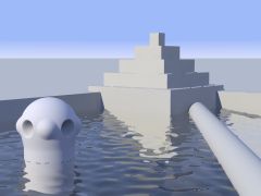
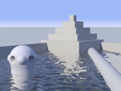
| Value=0.02 | Value=0.04 | Value=0.08 |
|---|---|---|
|
|

|
As you can see the water surface itself looks very much like with the
normal statement, but the interaction with the
walls is much more realistic.
The speed of this solution much depends on the function used, in this case it is still reasonably fast since the pattern used is fairly simple, but this can change with more complicated functions.
A different approach is to precalculate the surface geometry in the classical
form of computer graphics: a triangle mesh. In most situations the best method
to do this in POV-Ray is the heightfield object.
A heightfield can take a separate image file
or an internally generated matrix to define the positions of the triangles
which are placed in a rectangular grid. We use a pattern function like in the
isosurface version.
height_field {
function 400, 400 { fn_pattern(x, y, 0)*Value + 0.5 }
smooth
}
| Value=0.025 | Value=0.05 | Value=0.1 |
|---|---|---|

|

|

|
A heightfield is always 1 unit large so you have
to scale and translate it as appropriate. The 400, 400
specify the resolution of the mesh.
You can imagine that the mesh data requires quite a lot of memory and this is also the main disadvantage of this method. A large water surface reaching from foreground to horizon would require enormous amounts of memory. A possible solution would be not to use a heightfield and make a mesh of variable resolution.
realistic water structures
In the previous general samples i used a fairly simple pattern as an example. In reality the possible structures differ quite a lot. Sometimes we have very shallow parallel waves, sometimes very turbulent and splashy structures. Important factors that influence the style of the waves are - apart from the wind - the water depth, the rims and moving objects in the water like ships etc.
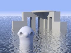
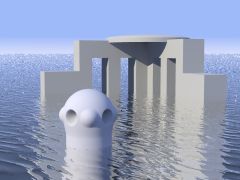
In the finish and interior samples i used a ridged multifractal pattern. This is well suited for quite strong ripples that are just before starting to splash. This pattern is not directional but linear structures can be obtained by overlaying parallel waves:
#include functions.inc
normal {
function {
f_ridged_mf(x, y, z, 0.1, 3.0, 7, 0.7, 0.7, 2)
+ sin(x*2.5)*0.4
} 0.8
scale 0.13
}
or asymmetric scaling:
#include functions.inc
normal {
function {
f_ridged_mf(x, y, z, 0.1, 3.0, 7, 0.7, 0.7, 2)
} 0.8
scale <0.13, 0.4, 0.13>
}
| plain | overlaid sine | asymmetric scaling |
|---|---|---|
|

|
|
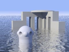
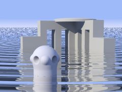
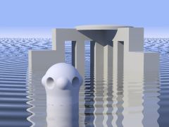
There are quite a lot of POV-Ray Patterns that are suited for water structures in some situation - either on it's own or in combination with others.
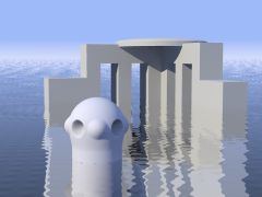
Here are some example of basic patterns:
| bumps 0.3 scale 0.1 | wrinkles 0.2 scale 0.2 | granite 0.15 scale 1.2 |
|---|---|---|

|

|
|
| waves 0.3 scale 0.1 | ripples 0.4 scale 0.4 | leopard 0.6 scale 0.04 |
|---|---|---|
|
|
|
Finally you can of course also try an accurate physical simulation. With taking into account all possible influences including interaction with the environment this can get extremely complicated. See the links section for some approaches in that direction.
If we restrict the situation to deep ocean without shore a simplified model is possible. It basically superposes a lot of sine waves with different frequencies and directions to a wave pattern. Distribution of frequencies and directions depends on the wind speed.
The description of a practicable model for those distributions can be found
in a
![]() paper on visualizing water surfaces (German).
paper on visualizing water surfaces (German).
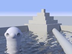
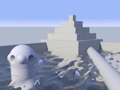
I wrote an implementation in POV, it generates a function that can be used in normals, heightfields and isosurfaces. The following samples show the results with different wind speed settings.
function {
Waves(pi/2, WindSpeed, 0, 650)
}
| WindSpeed=4.1 | WindSpeed=4.4 | WindSpeed=4.6 |
|---|---|---|
|

|
|
Since the function generated by the Waves() macro
is fairly long and slow, this method is less suited for isosurfaces.


