The well known Mercator projection ubiquitous in maps on the internet has one important property – it features a strongly varying scale across the area it is used for. This is why Greenland appears to be larger on the map than South America for example. Scale varies by a factor of more than 11 across the usual square cut of internet maps and even if you ignore the very north- and southmost parts in central Antarctica and the Arctic Ocean you have a scale ratio of 8 between the Equator and high polar latitudes.

In principle this is not a huge issue for internet maps since you can freely zoom in and out. This property of the projection was therefore accepted because of the huge advantages it provided otherwise. The problem is however that traditionally map design and geodata processing is not used to dealing with such variability in scale. In other words: while in principle everyone knows about this aspect of the projection almost everyone ignores it and pretends the web mercator map is just like any other projection.

One of the most obvious situations where this is the case are the countless data statistics maps, in particular the well known data density plots like Martin Raifer’s OpenStreetMap node density map – These are plainly wrong when considered a quantitative depiction of the data density.

They show data density in features per square meters in projected coordinates which is much different from actual square meters on the planet surface. And the difference is huge – when the linear scale varies by the factor of 11.5 between equator and map edge the density varies by the square of this factor, that is more than 130.

I put up a small tool on github that can be used to compensate for this difference in post processing. The tool is generic, it should work on any GDAL compatible raster format (where GDAL provides read/write support) with coordinate system information and on any projection (provided the inverse transform is known to proj4 which is also necessary for gdalwarp for example).

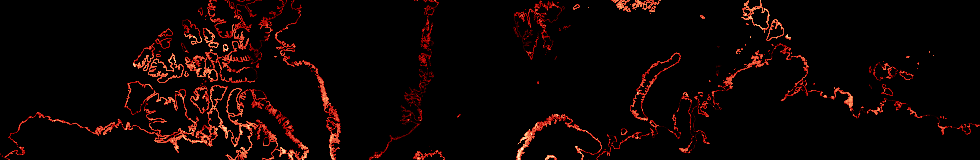
I demonstrate it here on the node density of an OSM coastline extract – not patient enough to run through a whole planet. For plotting node densities you can use the new node_density in libosmium Jochen implemented or my own gdal_nodedensity tool which also allows plotting way densities independent of the distance of nodes in the ways. Invoking gdal_nodedensity like this

gdal_nodedensity -a_srs EPSG:3857 -ot Float32 -ts 1024 1024 -te -20037508.342789244 -20037508.342789244 20037508.342789244 20037508.342789244 osm_coastlines_tmp.osm coast_nodedensity.tif

produces the following incorrect density plot where density is shown too low towards the poles.

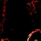
When you now run

gdal_valscale coast_nodedensity.tif

You get the correct density plot:

That’s it – no further parameters, all information is obtained from the image file.

Another program is available in the gdal-tools repository that buffers a raster mask by a certain distance – again in real world units rather than projected coordinates. Taking a coastline mask for example (produced from a coastline shapefile through gdal_rasterize --config GDAL_CACHEMAX 2048 -a_srs EPSG:3857 -ot Byte -ts 1024 1024 -te -20037508.342789244 -20037508.342789244 20037508.342789244 20037508.342789244 -burn 255 -at osm_coastlines_land_3857.shp coast_mask.tif – the -at ensures you do not miss any small islands):

You can run

gdal_maskbuffer coast_mask.tif 200000

and get a 200 km buffer of the coastline:

None of the common vector processing packages offers variable width buffering. If you for example apply ST_Buffer() in PostGIS you will get a constant width buffer in the chosen coordinate system, even when using the Geography data type, and when the feature extents across half the globe this will be wrong (see the warning in the above linked documentation). The only way you can achieve correct buffering in a global vector data set is by splitting all geometries into small enough chunks so scale variance does not matter any more for the individual feature and buffer them individually by the individually calculated distance. This is a lot of work and even that will fail when you want to buffer by a large distance where scale variation has an effect. You would then have to buffer in steps and split the geometries again in between…

gdal_maskbuffer currently only support isotropic scaling – proj4 would also support anisotropy but the CImg distance calculation only covers the isotropic case. It also does not take into account the periodic boundary conditions in x-direction. Both tools have only been tested for web mercator (EPSG:3857) but should work on other projections as well. gdal_valscale also currently unnecessarily loads the whole image into memory which could cause problems with large images (IIRC GDALDataset::RasterIO() does not support reading above the 32bit limit at the moment). Internally the tools invoke the pj_factors() function from proj4 to determine the required scaling factors which you can also have the proj tool report for individual coordinates.