Imagico.de | blog

October 5, 2022
by chris
0 comments

Autumn and spring in polar regions

In addition to the recent autumn colors images here two views of the polar region autumn and spring on the northern and southern hemisphere. The first shows the Ellsworth Mountains with a low sun position just after the end of the southern winter and the beginning of the observation season in September.

Ellsworth Mountains in late September 2022

The second one shows southern Baffin Island with the Nettilling Lake after the first show in early October.

Nettilling Lake in early October 2022

Both views are produced from Landsat 8 data and you can find them in the catalog on services.imagico.de.

September 30, 2022
by chris
0 comments

Blog moving

As you maybe have already noticed this blog has moved to a new location – from blog.imagico.de to imagico.de/blog. This is mostly to support also https connections (for which a separate subdomain is inconvenient). The move was made difficult by the blog location being not easy to change in WordPress. I now finally got around implementing that – together with an upgrade of the WordPress software, which is always quite a hassle meanwhile as well.

All links going to the old location should get redirected to the new place.

Hope everything works as before. If there are any problems please let me know in the comments.

September 22, 2022
by chris
0 comments

Autumn colors 2022

Autumn 2022 is starting on the northern hemisphere so here two impressions of early fall colors, the first from Kamchatka:

Shiveluch, Kamchatka in Autumn 2022

Shiveluch detail

The second from Canada, from the lower end of the Great Slave lake near Fort Providence where the Yellowknife Highway crosses the Mackenzie River:

Fort Providence and Mackenzie River in Autumn 2022

Fort Providence detail

Both are based on data from Sentinel-2 and you can find them in the catalog on services.imagico.de.

Eastern Himalaya by Landsat 7 on 2022-08-12

September 21, 2022
by chris
0 comments

Landsat 7 last images

According to plans announced some time ago the USGS is going to stop recording images with Landsat 7 at the end of September, ending routine operation of the satellite after more than 20 years.

Like EO-1 where i discussed this matter in more depth, Landsat 7 has run out of fuel to maintain its orbit and has started drifting to earlier morning recording times. This drift has not progressed as much as with EO-1 in 2017 yet but it is visible in the images recorded in the form of longer shadows quite well.

Eastern Himalaya by Landsat 7 on 2022-08-12

Eastern Himalaya by Landsat 8 on 2022-08-13

In addition the USGS has lowered the orbit of the satellite some time ago to make space for Landsat 9.

Landsat 7 is in particular noteworthy historically because it is Landsat 7 imagery that has shaped the public perception of Landsat as a source of earth observation images more than any of the other Landsat satellites. That is mostly because Landsat 7 was the newest Landsat satellite and the main source of Landsat imagery when the Landsat program moved to an open data distribution policy and during much of the period of popularization of Landsat data that followed (see the history of the Landsat satellites).

The strange thing about this is that Landsat 7 was struck by a major failure in its imaging system (known as the SLC failure – standing for scan line corrector) only four years after beginning of observations in 1999. The failure massively reduced the usability of Landsat 7 data for many, in particular for visualization application. So while the public image of Landsat has largely been formed by Landsat 7 recordings, it has predominantly been images from 1999-2003 that have contributed to that. These about 20 year old images are still widely used in popular map services these days, most notably Bing Maps, but also nearly universally by almost all map services for the Antarctic (though you can now get a more up-to-date alternative meanwhile of course ;-))

Malaspina Glacier by Landsat 7 on 2022-09-05

Malaspina Glacier by Landsat 9 on 2022-09-06

Technologically and in terms of image quality Landsat 7 is a bit of a relic from another time. Even compared to other satellites launched around the same time (like Terra in 1999 and EO-1 in 2000) Landsat 7 was using conservative technology for its imaging system, with only smaller improvements compared to what had already been used for Landsat 6 in 1993, which failed on launch.

The most significant constraint of Landsat 7 data in terms of image quality is the rather limited dynamic range of the sensor and as a result the high noise levels in dark areas and frequent overexposure in bright areas. The design tried to mitigate that limitation by offering two different amplification settings of the sensor which were chosen based on the expected brightness of the earth surface in the area. As a result of this limitation the USGS stopped recording areas with particularly high contrast (that is especially polar regions) and concentrated the recording capacity of Landsat 7 on the main lower latitude land masses.

Another noteworthy aspect of Landsat 7 was that its high resolution panchromatic spectral band extended across both the visible range and the near infrared, which made its use for producing high resolution natural color images difficult and subject to artefacts in case contrast in the near infrared is significantly different from that in visible light. It shares this characteristic with many higher resolution commercial satellite sensors – both back then but even today. You can see that in the images shown here comparing the appearance in Landsat 7 and Landsat 8 images.

Despite these limitations – for the needs of most data users it seems to have been fairly sufficient for most of the operational history of the satellite. The rather slow adoption of Landsat 8 by data users after 2013 pretty strongly supports this impression. In a way that is also the business model of Landsat overall so far – continuity before innovation.

Chersky Range by Landsat 7 on 2022-09-05

Chersky Range by Landsat 8 on 2022-09-06

The future of Landsat

Landsat 7 is being replaced directly by Landsat 9 in its orbit and therefore recording schedule. I have yet to write about Landsat 9 in more depth which i have not yet gotten around to. That means we now have a two Landsat satellite constellation with a combined revisit time of 8 days and with both satellites having almost the same capabilities.

What comes after Landsat 9 is still unclear. The most recent publicly available update i could find is here – but this is not providing much more in substance than this and is still rather vague and at the same time it is unclear to what extent what is presented there as what will be (which in a nutshell looks very much like a Sentinel-2 clone with additional spectral bands) is actually already decided on the actual decision making level. In particular everyone should keep in mind that during the early considerations for Landsat 10/Landsat Next the idea was discussed to depart from the full open data model. And there is no clear statement so far that this is not under consideration any more. The existence of Sentinel-2 makes this somewhat unlikely (because with a free alternative there would not be much of a business case for non-free data in a very similar quality and timeliness range). The 10m resolution number that has been widely communicated as target around future Landsat systems is interesting in that regard because this is what now – thanks to Sentinel-2 – is the division line between what is available as open data and what is only commercially available. If Landsat does not go beyond that the status quo would be kind of preserved. If Landsat would move to higher spatial resolution, however, that would massively cut into the domain of commercial satellite operators. In other words: It would probably be politically unfeasible for Landsat planners to try going beyond 10m spatial resolution.

On the other hand a future Landsat with a 10m base resolution would mean an increasing gap between low and high resolution systems with nothing in sight so far to bridge that gap. Let me explain: Over the past decades (essentially since 1999) the main global open data visible light image sources we had were:

MODIS (since 1999/2002, near daily coverage at two times of day) at 250m resolution
Landsat (since 1999, every 16 days – 8 days with Landsat 5/7 and after Landsat 9 became operational) at 15m reolution (30m multispectral)

With both MODIS satellites reaching their end of life now and no direct replacement being planned we will in the future have from the US:

VIIRS (since 2011/2017 + another planned for 2022, daily coverage at 2(3) times of day) at 375m resolution
Landsat Next (probably 2030+, probably less than one week revisit interval) at 10m resolution

From the EU we have in addition:

Sentinel-3 OLCI with near daily coverage at 300m resolution
Sentinel-2 with 5 day revisit (but no complete recording of all land masses in practical operation) at 10m resolution

There is not much in between though, just the Japanese GCOM-C at 250m resolution and Amazonia-1 from Brazil at 60m resolution (which is not operated for world wide recording apparently). But neither of them offers a substantially better revisit frequency than the two satellite Sentinel-2 constellation. This means as a data user you practically have to either work with a resolution of 375m or 300m or go to a much higher resolution but deal with the disadvantage of a a low recording frequency and a large data volume to process.

September 3, 2022
by chris
0 comments

Thoughts on the OpenStreetMap data model

In this post i want to write a bit about the OpenStreetMap data model. This has obviously been influenced by the discussion in the OSMF to make changes to that model i already mentioned in a previous post.

I am a bit reluctant to write about this here and i want to explain the reasons for that first. I am writing about this out of intrinsic motivation. On the one hand for the intellectual challenge of discussing a highly complex interdisciplinary topic. It involves engineering aspects obviously but also natural sciences (in the form of the physical geography that a large portion of the OSM data represents) and social problems (through the role the data model plays in social interaction in the OSM community). On the other hand i also believe that my thoughts on the matter can be valuable considerations for the OSM community so sharing them publicly could be of benefit for the project.

However, the OSMF has started the public discussion of their plans to make changes by moving the whole matter on the commercial level (by commissioning a paid study on the subject). That means taking part in the discussion with the OSMF on the matter will inevitably involve engaging in discussion with people who have economic motives for representing their views. While i do not categorically reject doing that (doing so can still provide better insights into the subject and can be of benefit for the OSM community at large), we are in the field of diminishing returns here. Pro bono fighting an uphill battle against economic interests, defending my views not against arguments and reason but against people who have an economic interest not to change their view, is not a sustainable strategy in any way and is typically not in support of what i described above as what motivates me to write about this matter here.

Long story short: I am writing this not to engage in a discussion with the OSMF of their commercial project to change the OSM data model but to have an open intellectual exchange with anyone interested in the hope to advance our collective understanding of the subject and to educate people who are interested in aspects and context of the topic they might not be aware of.

Writing this while knowing that many of the people who have the most influence on how the OSM data model will develop are – based on past observations – not very likely to be open to arguments and reasoning that challenge their views on the matter is painful – hence my reluctance of doing so. I still do this because i know that quite a few people in the OSM community are interested in diverse views of topics like this and value being confronted with ideas and perspectives especially also if they are different from their own.

So much for introduction – let’s get on the subject.

What is the OSM data model?

I want to start by defining what i want to actually talk about – because that seems to be quite a bit different from what is being discussed in the OSMF.

The OSM data model i want to discuss here is the form in which mappers engage in the act of mapping in OpenStreetMap. Technically it is the data format of the OpenStreetMap API. That is the interface through which mappers receive data from the central OpenStreetMap database and through which they submit back their changes of that data to the project.

On the social level the OSM data model is the language in which mappers in OpenStreetMap from all over the world perform the act of cooperative mapping. No matter what kind of tools a mapper uses or in what human language the UI of that tool is labeled, the OSM data model is the underlying common standard based on which mappers communicate through the act of mapping itself. That should give a bit of an idea of how fundamental it is for the functioning of the project on a very basic level.

The OSM data model is neither necessarily the format in which OpenStreetMap data is distributed to data users (which at the moment happens to be the same) nor is it necessarily the same format in which data is stored in the central OSM database (which at the moment is close to the API data model – though there are smaller differences – like the form in which coordinates are represented).

How does the OSM data model currently look like?

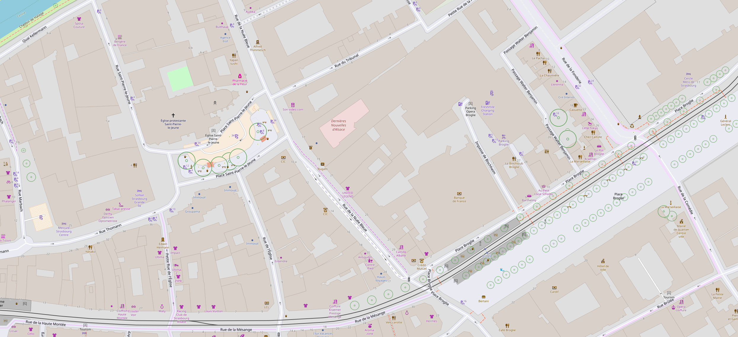
The OSM data model is – in its basic paradigm and compared to other common forms in which geo-data is represented – a very generic, low level format. If i try to describe that in relatively simple terms i get:

Geographic locations (positions on the surface of the earth) as the fundamental components of geographic information are represented with so called nodes with coordinate pairs (latitude, longitude) as attributes.
Relationships between different objects and concepts that are modeled with more than a single geographic location are represented by so called relations – which contain references to other objects, potentially in a certain order and potentially with a certain role.
Sequences of geographic locations in a certain order can also be (and are widely) represented by so called ways which contain references to nodes.
All of these fundamental objects can have any number of attributes in the form of free form key-value pairs – so called tags.

Most of this data model is – as mentioned – very generic. That means it makes only very few assumptions about the way geographic information is represented beyond the basic paradigms of geography itself. It is beyond doubt that this characteristic has largely contributed to the success of OpenStreetMap over the past >15 years. The positive effect of the generic nature is usually seen primarily in the free form tagging system. But that is mostly because the OpenStreetMap mapper community has concentrated on that in their activities and is mostly using tags to develop innovative ways to represent geographic information. Many of the other advantages of this model are so far severely underused and i will get to why that is the case further down.

What are the issues with the current model?

I think i already indicated in the way i presented the current OSM data model above that the concept of the ways is kind of an outlier in the model. With the plans of the OSMF in mind i would go a step further and speak of the ancestral sin of the OSM data model.

First of all ways as a concept are superfluous in the OSM data model, a relation can be used to represent what is represented with a way just as well. Or you can look at it the other way round, a way is just a hard-coded and technically more restrictive type of relation:

it can only have nodes as members
it can not have more than 2000 of them
the members cannot have different roles

Beyond that ways are severely under-defined. Ways are usually interpreted to represent a sequence of straight line segments between its member nodes – but nowhere is it defined what that actually means. The most natural interpretation would be to consider the straight line between two nodes to be the shorter segment of the great circle running through those two nodes. Most tools processing ways however interpret a straight line to be a straight line in equirectangular projection (that is geographic coordinates interpreted as cartesian) or in Mercator projection – but that is not defined or documented in any way. If ways were just a type of relation defined on top of the basic OSM data model through consensus in the OSM community and could equally be changed or amended in their meaning through revised consensus, that would be different – we have plenty of similarly under-defined concepts in tagging schemes and relation types in OpenStreetMap. But as a hard-coded element of the low level data model this is highly problematic.

The other main technical or formal issue of the model is that nodes can have tags. Discussing this could get us quite a bit into an abstract philosophical domain. I will try to keep it brief but be aware that this is going to selectively only present some of the arguments.

There is a continuum (or an infinite number of) geographic locations on the planet obviously. That act of mapping consists essentially of two parts:

identifying locations which have meaning.
documenting what meaning these locations have.

These two activities are not necessarily identical and the same location can have meaning in different contexts – for example a location at the corner of a building has both meaning as a point on the corner of the building as well as one end of the artwork painted on the side of the building and as a (concave) corner of the pedestrian area surrounding the building. That the OSM data model separates these two activities by separately recording the geographic location (the node) and the meanings it has (by being a member of ways/relations representing building, artwork and pedestrian area in the mentioned example) is one of the huge advantages of it. But this is only the case when the meaning is represented through ways or relations. When you have for example a path (way with highway=path) crossing a fence (way with barrier=fence) with a gate (node with barrier=gate) the node doubles as a location and as a carrier of meaning. That is not ideal because the two mapping activities described above are then not separately represented in the data.

Both of these issues are things you can hardly blame anyone for retroactively because they are the result of the historic development of the data model.

The OSM data model would improve a lot in its inner consistency as well as in practical handling if these two issues were fixed. That means the new data model would look like this:

Nodes would just contain coordinate pairs and have no tags, Real world features that are to be modeled geometrically with a single coordinate pair would be represented with a relation with the single node as member.
Ways would be eliminated and converted to a type of relation.

I am of course not the first one to identify these two things as key points where the OSM data model can be improved. Ilya for example mentioned these ideas recently independent of me. Most who analyze the OSM data model from the perspective of mapping will likely come to the same conclusion (or have done so in the past already).

Are these the only significant issues with the OSM data model that are worth addressing? Probably not. There are quite a few further things, mostly related to the way changes in the data are being represented and managed (with versions and changesets – things i kept out of the description above). But to keep things simple i intend to limit this post to matters of representation of geographic knowledge itself.

The struggles of working with a generic data model.

Of course the structure of the low level data model is only half of the story.

The other side of the topic are the difficulties resulting from having such a generic and low level data model as we have in OpenStreetMap for the process of building consensus on how we practically document geographic knowledge with that data model.

Again this topic is historically mostly discussed in the context of the free form tagging system in OpenStreetMap – which is the practically most visible unique characteristic of the OSM data model compared to ways to represent geographic information elsewhere. There is consensus that the free form tagging system was and is an important basis for OpenStreetMap having developed the way it did (in the positive sense). But, as i already discussed in a different post, this has also resulted in problems, and as OpenStreetMap grows it is going to be of fundamental importance to have a meaningful discussion on how the development of tagging in OpenStreetMap can scale and continue to function in a growing and increasingly diverse OSM community. I presented Tagdoc as a sketch for what i think would be a valuable component to facilitate better understanding and as a result more qualified decision making in tagging and tag development.

There is a subset of tagging that is of fundamental importance so that OpenStreetMap is able to use its innovative data model to its true potential and the OSM community’s struggles to actually develop a meaningful discussion and consensus building process on that has significantly kept back OpenStreetMap for more than a decade.

This subset of tagging i am talking about are the relation types. As i outlined above, relations are the core feature of the generic OSM data model to implement higher levels of abstraction to represent concrete geographic knowledge.

Technically relation types are just tags. But the social dynamics around them in the OSM community are very different from normal tags.

For normal tags the conventions how they are used and interpreted are influenced primarily by the following actors:

mappers through the use of the tags.
wiki activists (people engaged in editing of tag documentation on the OSM wiki and participating in proposal processes).
editor developers through decisions they make with tagging presets.
map style developers through decisions what tags to interpret and how to interpret them.
other data users through their tag interpretation practice.
QA tool developers.

For relation types the primary influences are very different:

editor developers through decisions for what types of relations they offer an editing interface to.
developers of data interpretation tools through decisions which types of relations they support and how they interpret them.
to some limited extent QA tool developers.

As you can see there is a fundamental difference. The practical use and meaning of tags is influenced by a wide range of actors with different backgrounds. This sometimes leads to chaotic situations – which some people despise and call for more authoritarian tagging paradigms. But overall it has served OpenStreetMap quite well – even if there are and continue to be problematic concentrations of power and influence in that system as well.

For relation types however there is a clear gatekeeper role of a very small set of people who practically decide (though they might not actually be aware of that) which relation types are ‘permitted’ (and as a result are practically used in significant volume) and what the mapping conventions are for those. And all of these people are software developers.

As a result of this we essentially have only a handful of relation types in OpenStreetMap that are (a) practically used in significant volume and that are (b) used with a significant level of consistency that allows data users to interpret them in a meaningful way. And all of those have been around already for more than ten years now.

This is the big practical problem in my eyes. In contrast to tags where the power and influence on conventions is widely distributed and grassroots inventions of new tags have a reasonable chance to be successful (and where separating good and bad ideas by mappers voting with their feet usually works) this is not a working mechanism for relation types. This cripples the OSM community’s ability to develop the way it maps the world wide geography in an innovative fashion and prevents it from making full use of the potential of the data model. This is not a problem of the data model itself but stems from the low level nature of it, making it necessary to develop higher level conventions on top of it – which the OSM community is, one a social level, currently unable to do.

This is a hard problem to solve and I have no solution for this to present here. But i know what is no solution: To give up and to move from the generic and low level data model we have to a constrained higher level model of points, linestrings and polygon geometries.

There are quite a few secondary problems that have turned up as a result of the OSM community essentially having been unable to advance on the development of relation types – or of other higher level conventions for representing geographic relations. One prominently visible problem is the overuse of multipolygon relations for representing concepts that could be represented much more efficiently and easier to maintain otherwise. As a simple (though maybe somewhat tongue-in-cheek) example: Think of large islands (like Greenland or Madagascar). These are currently represented in OpenStreetMap with very large multipolygon relations with thousands of member ways. These multipolygon relations however contain almost no information at all that is not already in the database otherwise. If you’d transfer the tags of the relation to a node – either anywhere within the island or on its coastline – that would contain all the information already in a much more compact form. I am not necessarily saying that this is a change that should be made specifically for islands, arguments could be made for keeping the relation here, even from a mapper perspective. My point is that the OSM community currently lacks the fundamental ability to make such a change (or any substantial change in higher level mapping conventions beyond the atomic tagging of individual features). And this is essentially a different side of the same problem. Technically fiddling with the low level data model will not help with that.

What about the other problems?

If you have read the report on changing the OSM data model commissioned by the OSMF you might wonder why so little of what is identified there as problems is discussed here and why most of what i discuss here is not of much importance in that study. That is because i look at the OSM data model purely as the language in which mappers communicate and exchange their work while that study:

is almost exclusively concerned with the needs and the difficulties of global scale data processing on the data user side,
makes the up-front assumption that the mapping data model and the format of distribution of OSM data en bulk to the data user necessarily need to be identical and
essentially proposes to eliminate the function of the OSM data model as the language of exchange between mappers. Instead it suggests that the data editing tools create an abstraction layer between the data format of the API and the paradigms of representing geographic information used by the mappers.

This is the wrong approach in my eyes. The solution to issues on the data user side in processing OSM data on a global scale is simple: Distribute the data in a form that avoids these problems. Doing so would probably be simplified quite a bit if the changes to the OSM data model i sketched above (elimination of ways and of tags on nodes) would be implemented. Also the problem of the two different means of representing polygons with closed ways and multipolygon relations would be eliminated by that.

Where we need to work on solutions is the social problem of developing and maintaining higher level conventions on top of the low level data model OpenStreetMap is based on. That is not an engineering problem of course. While technical means and tools are likely to be useful in implementing solutions to that once we have identified and agreed on them, people with technical skills and qualifications should resist the urge to focus on the hope of finding primarily technical solutions to this. That is not going to work.

Conclusions

That was – despite having grown to a lengthy text again, as you have become quite used to from me probably – a very quick run through a rather complex interdisciplinary topic that only scratches the surface obviously. That means it is going to be easy for people who want to selectively maintain a different perspective on the matter to dismiss my thoughts as too superficial. And that is fine. But make no mistake: That i try to present the topic in a brief and condensed (and hopefully not too cryptic) way does not mean i have not thought it through more in depth. Those who have discussed the OSM data model with me in the past know that i have always approached the topic with an open mind. And i still do. I present no solution that i claim is the right one, i merely present an analysis of the problem.

The main points you as a reader should probably take away from this post are:

If you look at the matter from the most important side to consider – that is from the perspective of mapping – it looks very different from how the OSMF seems to so far have looked at it.
The main problems are not with the technical structure of the OSM data model (though there are some quite obvious things where this could be improved) but in the ability of a massively growing and increasingly diverse OSM community to productively use the possibilities of the data model to be innovative and efficient in cooperatively mapping the world wide geography.

August 17, 2022
by chris
8 Comments

Over engineering

In the past years i have more and more moved to post my commentary on political developments in the OpenStreetMap Foundation towards the end of the year before the OSMF board elections instead of timely commentary of things as they are happening during the year. I am going to make an exception here by writing down some observations and thoughts on more recent trends and developments i consider particularly noteworthy.

If you have followed some of my more recent OpenStreetMap related posts here you might have observed that i have put an increasing emphasis on pointing out that the value put in the OSM Community on technical work in contrast to non-technical, in particular intellectual work, is quite seriously out of balance and that this is increasingly affecting the OSM Community’s ability to handle the various challenges it faces.

The recognition of this trend and its effects on my side has been emphasized in particular also by the OSMF more recently moving strongly towards an increasing dominance of technical interests and viewpoints. On the level of the OSMF board this in particular manifested in the departure of Allan Mustard from the board end of last year. Allan was the last remaining board member with a distinctly non-technical professional background. Everyone on the board now has a technical professional background and most more specifically in the domain of IT and software development. Allan’s departure from the board is of course not the singular cause of this shift in the OSMF, this is more the conclusion of a long term trend overall which – on the board level – started much earlier with people with a broader non-technical perspective on the board increasingly resigning and the OSMF membership increasingly electing people with technical backgrounds.

At least to me it became increasingly clear in the last months how much of a paradigm shift this is and how much of an impact on actions and decisions of the OSMF this could have in the future.

Beyond the composition of the OSMF board this trend is best visible in form of the shift in expenses for paid work. Until late 2020 the OSMFs main regular expenses for paid work were administrative assistance and accounting. This has completely shifted by contracting a software developer for iD and hiring a sysadmin since then. The exact amounts of money spent here are not known (contracts are not published any more and we will probably have to try to reverse engineer this info from the financial reports at the end of the year). In addition there has also been an increasing volume of non-regular paid technical work (in particular the three hand picked projects in the aftermath of the microgrant program). The newly revived Engineering Working Group now has a EUR 50k budget for paid work – the highest of any working group after Operations if i am not mistaken.

A project of the Engineering Working Group is also what i want to discuss in more detail here. Earlier this year the EWG has decided to contract a study for changing the OSM data model.

The specific details and motives for this are unclear – the minutes do not reveal substantial information on that. What we know is that this study was contracted through single tender action (the contract terms are not disclosed, not even the exact aim of the study) and not through the EWGs project funding framework.

The study the EWG has contracted has now been published and this is what i want to discuss a bit more in depth here. I am not going to comment on the technical aspects in substance but i want to share a few thoughts on the economic and social context of the whole thing.

I am – by education – an engineer myself, with a master and a PhD in mechanical engineering. During my early years in engineering i had – like many other engineers – a tendency to look down on consulting companies doing feasibility studies and receiving quite significant amounts of money for those while having no real street credibility so to speak in the domain of engineering. Furthermore these consulting companies often did not predominantly seem to employ engineers but people with a background in economics or social sciences.

This negative view of the young engineer in me has significantly changed since then. And in case you wonder: This change has happened already before i became a consultant myself ;-). While i think many larger generic consulting companies (which is what many people have in mind when they hear the term consulting) have very questionable business practices and models, i meanwhile have a significant appreciation of the work of smaller specialized consultancies, in particular in producing feasibility studies, and consider their role in our society with its highly specialized competencies and division of labour to be quite essential.

My impression is that what the OSMF apparently did here is the approach of a naive young engineer towards doing a larger project: Contracting an experienced engineer with practical work experience in implementing this kind of project for a feasibility study with the aim to find out how they can make the project work.

There are very good reasons why this approach is not typically taken.

One obvious reason is that the contracted engineer has, if they are also a likely candidate for being contracted to implement the project, a clear conflict of interest. This is one of the main reasons why feasibility studies tend to be done by independent consultancies who have no stake in the actual implementation of the project.

The second important reason is that in most larger engineering projects the main risks and obstacles are typically not technical in nature. To truly assess the feasibility of the project, the risks involved and the resources required, you need experience outside the domain of engineering. You need to regard the broader social and economic context of the project. This is one reason why consulting companies frequently employ social scientists and humanists.

I am not sure if it is realistic to expect people in the EWG and on the OSMF board to realize they took the wrong approach here and recognize the need to revise that. But i know that there are plenty of people in the larger OSM community who have a broader perspective on the matter and who will therefore likely be interested in a more critical commentary on the approach taken to this project here. In any case i thought it is prudent to make this comment early to give everyone the chance to consider it.

What impact does this have on the actual matter of the OSM data model and its future development? I obviously have my thoughts on that too. But this is beyond the scope of this blog post.

August 11, 2022
by chris
13 Comments

State of the Map 2022

In about a week the OSMFs State of the Map conference is going to start and to avoid anyone looking for me in vain there (i have been at the last four State of the Map conferences – the last two of which were virtual events) – i am not going to be there this year.

This has multiple reasons, one of the most relevant being that this year’s event is – more than in any of the last four years – an event quite ostentatiously targeted at wealthy people and people whose visit is paid for by a third party. It is perfectly fine to have such an event, and i wish everyone at the conference an enjoyable and successful time, but this makes it much less attractive for me to visit.

With the strong limitations of the last two years to meet in larger groups, i would this year have liked to meet in person with various people involved in OpenStreetMap whom i could not meet in the past years, including quite a few who are likely going to be in Florence despite the fairly steep costs of a visit there during the height of holiday season with hotel and travel prices at their peak. But to be frank – what i enjoyed most in previous years was in particular meeting and talking to economically more marginalized people.

I played a bit with the idea of visiting Florence but not going to the commercialized conference and instead just meeting with people outside the organized event and visiting and getting to know the city otherwise. But as said there were other reasons speaking against it and also, while i could have afforded a visit to Florence in August, that is not equally the case for many other people active in OpenStreetMap. And choosing Florence in August as the place and time where people from the OSM community have the chance to meet me in person would also have made a statement as to whom i am mostly interested in meeting, even when done detached from the SotM conference.

In past years i repeatedly have criticized that affordability of the visit is not a criterion in the planning of the conference, not even on paper, and neither for picking the place nor for picking the date of the conference. This fact is of course perfectly in line with the OSMFs diversity statement – which disallows discrimination by almost anything, but quite explicitly not by wealth.

Anyway – for those in the OSM community who would like to meet me in person – i plan to be at the Karlsruhe Hack Weekend in September, after also having been absent there for the past two years. Despite the limited number of participants allowed, there is still room for people to come there, Karlsruhe is just a two hour train ride from Frankfurt Airport and there is a good selection of decent and affordable places to stay in Karlsruhe.

I also generally look with interest at the announcements of any other events in the OSM community that have been planned with the visible intend and desire to be affordable and accessible also for less wealthy people and being truly welcoming for a diverse audience in the original sense of the word. For the past two years the options to visit such events have been rather limited, but i hope this will get better in the future again.

Florence in Spring 2022

June 5, 2022
by chris
1 Comment

Concluding remarks on tree rendering

This is part four of a four part series of blog posts on the depiction of trees in maps – see part 1 for a discussion of tree rendering in traditional maps and plans, part 2 for mapping of trees in OpenStreetMap and rendering in OSM based maps and part 3 for the discussion of a new concept of tree rendering.

The tree rendering implementation i showed and explained in the previous part is essentially just a sketch demonstrating a few of the design concepts you can explore once you truly disregard the technical constraints of common automated map rendering tools. Is this too much for a general purpose map style? Maybe.

As i mentioned recently again the whole world of automated rule-based map design is, once you leave the pre-made paths scouted already by tech companies and tool developers working for them, largely unexplored territory. Working on the tree rendering once more made me realize how much that is true especially for large map scales and high zoom levels. Once you start truly designing maps specifically for z19/z20 you are well into the traditional domain of architectural drawings and site plans – which is a whole new field of considerations and design ideas, as i tried hinting at in the first part with some examples. Most digital interactive map designers so far simply treat this scale range as an extrapolation of the smaller scales. This even more applies to all the modern vector tile maps where everything above z16/z17 is literally just the same rendering blown up to larger scales plus more POI symbols and labels.

And i think this series of blog posts also once more demonstrates that the inherent, high level capabilities of currently available map rendering tools are very limited compared to what in principle would be possible and desirable to have to produce well readable maps. The CartoCSS + Mapnik toolchain i use here has the advantage that it provides the means (via PostGIS code) to implement this on a low level by hand but practically such low level techniques are probably beyond reach for many map designers. And using this method has its own limitations – apart from the obvious efficiency issues you also cannot combine this kind of manual symbol processing with use of symbol/label collision detection and prevention for example.

So once again my strong suggestion to the OSM and the FOSS community that i have already stated on various occasions: You need to strategically invest in advanced map design tools for automated rule-based map rendering. And if you do so while looking at things purely from a software developer perspective or following the footsteps of big tech companies you will fail. The proprietary software producers have learned this lesson. They actively involve and actively listen to map designers in their strategic planning and research. Their target users so far are predominantly still the traditional map creators to whom map design means manual processing of concrete data and not the development of automated rules to process generic data like i discuss it here. But this is going to change. So do not miss this window of opportunity.

June 3, 2022
by chris
5 Comments

A new design for tree rendering in digital maps

This is part three of a four part series of blog posts on the depiction of trees in maps – see part one for a discussion of tree rendering in traditional maps and plans and part two for mapping of trees in OpenStreetMap and rendering in OSM based maps.

Based on what i discussed in the first two parts of this series of blog posts, i have contemplated and experimented with new ideas for rendering trees in digital maps for quite some time. In the alternative-colors style i had already reverted the removal of tree depiction from z16 and z17 earlier. Since trees are important for many map users and mappers evidently invest a lot of time and energy in mapping them, degrading them to a POI of local importance is not a good idea in my opinion.

But the problems with the existing rendering in OSM-Carto otherwise remain:

The transparency in rendering is not working well on the higher zoom levels (z18 and z19) where it applies to a larger area.
The symbols use a lot of space and affect readability of the map, in particular in areas with dense presence of trees and this could even discourage mappers from mapping all trees in some cases. At the same time it is wasteful because it transports no information beyond the simple here is a tree while – as discussed in the previous post – mappers use all kinds of secondary tags to further characterize trees which could well be used for more differentiated rendering, in particular at the higher zoom levels.
These problems will further aggravate if you’d want to extend the style to higher zoom levels.

I contemplated the idea of using profile symbols, because – as discussed – this is very common in traditional maps and it allows transporting differentiated additional information on the type of tree. However, this approach would not work too well at larger scales/higher zoom levels. And it does not provide very precise information on the position of the tree. As i showed, large scale plans typically use from-the-top view depictions and have developed a lot of useful design concepts in that domain. If you want to have a useful depiction of the tree size at these scales there is really no alternative to a from-the-top view.

The basic design concept

The basic design idea i have now implemented is using from-the-top view symbols in a line drawing design. If the symbol design is not too dense it allows features below the tree symbol to be visible through the line drawing – while being less distorted in coloring than with the semitransparent fill color of the OSM-Carto design.

Tree depiction using line drawing symbols – left at normal scale (z19), right at double resolution rendering

Zoom level progression of basic `natural=tree` from z16 to z20
z16	z17	z18	z19	z20

The difficulty is how to deal with symbol overlaps. I definitely wanted to retain the feature of tree symbols being non-blocking because trees frequently exist in dense groups and just rendering one of them in such cases is highly non-ideal. And in areas where there are a lot of POIs (like in dense urban environments) most trees would not be rendered if they were blocked by other symbols.

If you’d naively show line drawing symbols with overlaps you would often end up with a dense, non-discernible mess in areas with dense presence of trees. The technique of applying layer based opacity in OSM-Carto successfully avoids that – but only for a uniform fill color. I considered applying a structure pattern to a polygon aggregated from the buffers of the individual trees (a bit similar to the rendering of unpaved roads). But that would look rather crude for trees and would evidently be a solution just chosen because it is technically simple and not because it is good design.

The samples from architectural drawings and site plans i showed in the first part demonstrate a number of techniques how overlapping top view tree depictions can be handled graphically. None of the automated map rendering tools i know of has any kind of built-in support for anything like that though. What i ultimately ended up with is implementing the whole symbol drawing in PostGIS. This is certainly not very efficient (doing this at the compositioning level of the renderer rather than at the geometry processing stage would be much faster probably) but it is doable.

To make that possible, all the symbols were entered into a distinct database table as PostGIS polygon geometries and are then processed to generate the desired shapes to be then rendered just as if they were mapped geometries from the rendering database. This probably sounds more complex than it is in principle – though the geometry processing is certainly non-trivial. The route to get SVG symbols into a PostGIS database is via conversion to PDF using inkscape and then using OGR basic PDF support (with OGR_PDF_READ_NON_STRUCTURED). As an alternative route of symbol generation for simple abstract shapes i also implemented support for generating them using PostGIS code. Both routes can also be combined to supplement/edit a file based symbol with a PostGIS query. This is in particular useful for dynamically scaled symbols – as i will discuss in more detail below.

Handling of overlaps between tree symbols

Tree type depiction

As you could already see in the examples so far i designed different symbols for different types of trees. This is less easy to do in an intuitive fashion than for profile symbols but it is still manageable at least for the basic leaf_type and leaf_cycle classes.

Tree symbols differentiated by leaf_type/leaf_cycle at z16 to z20

At z16 and z17 trees are – like in OSM-Carto before 2017 – rendered with a plain green dot. At z18 trees start being differentiated by leaf_type and from z19 on also by leaf_cycle. The illustration of deciduous leaf_cycle takes the form of a display of the major branches and trunk of the tree (as visible from above in the absence of foliage) or a cleared center area in case of the needleleaved symbol. The lack of a specified leaf_cycle is illustrated with a small circle in the center of the symbol. Palms (genus/taxon=Arecaceae) are shown with a distinct symbol (independent of the leaf_type/leaf_cycle tag).

Tree sizes

The other main feature for individual tree rendering i implemented in addition to the leaf_type/leaf_cycle depiction and the customized handling of symbol overlaps is dynamic scaling of symbols according to recorded information about the tree size.

Trees vary greatly in sizes – what is commonly mapped in OpenStreetMap as natural=tree might have a height of just 2-3m for a small ornamental tree up to more than 50m. Canopy diameters (diameter_crown) can range from a meter or less up to around 50m as well. Such information is not recorded for a large percentage of trees mapped in OpenStreetMap but in absolute numbers it is still quite a few that come with such data. And visualizing tree size information in the map at the higher zoom levels would increase the usefulness of tree rendering quite significantly.

With the top view visualization i have chosen here a natural way to visualize the tree size is by varying the symbol size based on the canopy diameter. This is also the way large scale site plans often differentiate trees – as i have shown in the first part of this blog post series. Just scaling the whole symbol however does not work very well for that. For a line drawing symbol, scaling the line work while maintaining the drawing width would be a possibility – that is what most of the mentioned site plans do. However this still can lead to the problem that smaller symbols would have a too detailed geometry while larger symbols are not detailed enough. I tried and implemented both the approach to design distinct symbols for different rendering sizes and to have parametrized symbol geometries that scale according to non-trivial rules. Here is how this looks like:

Trees with different diameter_crown values at z18 – click to see z19

To inspect the symbols in the symbols table i also created a separate map style file (treeinspector.mml) that visualizes the content of the symbols table as is. Here is how this looks like:

The symbols table inspection style

The symbols for palms exist only for the sizes they have been designed for. The renderer then picks the closest match in size and scales it to the tagged tree size, rounded to the next integer pixel size to ensure pixel alignment as far as possible. For the parametrized symbols (most of the larger ones) a separate symbol is pre-generated by the generate_symbols.py script for every integer symbol size. This is either fully generated by PostGIS SQL code (for the unknown leaf_type symbols on the right) or composed of a scaled SVG based design and additional parametrized modification via PostGIS (for the known leaf_type symbols). As you can see the overall size of the symbols are scaled while the line with of the abstract circles and the geometry of the center symbol is not in the same way (for larger symbols this also gets increased moderately). For the larger symbols with know leaf_cycle the center portion (indicating the leaf_cycle) is rendered at a constant size while the outer rim (which does not change with leaf_cycle) is scaled according to the symbol size. The definition of all these symbol generation rules can be found in symbols.yml.

In the above symbol table only odd sizes (in pixels) are shown above 17 pixels. Only those are used for the individual tree rendering to ensure a uniform pixel aligned rendering at different sizes. For the tree rows (see below), where the symbols are not pixel aligned, also the even sizes are used.

In case diameter_crown is not mapped for the tree an estimate is made from either the height (0.3 times the height) or the trunk diameter (5 times the diameter). This is implemented in the function carto_tree_diameter_mapped(). As with other cases of ground unit rendering i implemented in the alternative-colors style, the symbol size is chosen as the maximum of the default symbol size for that zoom level and the size as tagged or estimated based on tagged height or trunk diameter.

With the shown technique to cut out overlapping tree symbols there is also a possibility to indicate different tree heights separately to some extent by having the height define the drawing order. If the height is not tagged, the drawing diameter of the tree symbol (determined as described above) is used to define the drawing order instead. That of course means that small trees completely under large ones are hidden.

Overlapping tree symbols, ordered by tree height (at z19, with varying diameter_crown as well) click for double resolution rendering

Tree rows

One part of this tree rendering project i struggled quite a lot with are the tree rows. This is to a large extent because natural=tree_row is a fairly ill defined concept in OpenStreetMap. As mentioned in part 2 there is no established tagging to indicate the spacing of trees in a tree row and neither is there a clear agreement what qualifies a set of trees to form a tree row. A tree row might be

four trees spaced 50 meters apart but planted evidently in a collinear fashion so forming an abstract row while not in any way forming a continuous object.
trees along the edge of a road or stream which might have originally been planted in a systematic fashion but with – at present – irregular intervals between them.
a dense arrangement of trees along the side of a agricultural plantation serving as wind protection.
a regularly spaced line of trees in a tree plantation for agricultural purposes.

All of that might indiscriminately be modeled with natural=tree_row in OpenStreetMap. Visualizing that in a way that properly represents all of these cases in a decent fashion is next to impossible.

The traditional rendering in OSM-Carto is taking the simplistic approach to simply align the design directly to the data model. By rendering individual trees as a buffered point and rendering tree rows as a buffered line. While that is a reasonable choice to give the mapper very direct feedback to what they have mapped, it does not provide much support or guidance regarding the semantics of that mapping.

The approach i ultimately chose for tree rows is to render them like a line of individual trees with a relatively dense arrangement of individual tree symbols. But the cutting out of the individual tree symbols against each other is done in a different fashion, not prioritizing one symbol over the other but cutting them at the bisector between them. I am not sure if this is the best solution. But it is one that harmonizes quite well with the individual tree depiction and at the same time makes the results easy to distinguish from a line of trees mapped individually.

Tree row rendering with different tagged width values at z18

Zoom level progression of basic `natural=tree_row` from z16 to z20
z16	z17	z18	z19	z20

For efficiency in rendering – since all of this has to be done in SQL code on the fly – the individual tree symbols of the tree row are only cut against the previous and next point on the line which leads to some overlap artifacts in case of sharp corners on the line.

Tree rows with sharp corners at z19

Some might wonder why i have not used a line pattern to generate this kind of visualization. There are multiple reasons for that. First: line patterns in Mapnik don’t have support for line caps – which would not work very well for this use case. Second: Line patterns are drawn continuously along the length of the line and no special attention is given to corners in the line geometry. What you’d want, however, for tree rows (and especially also hedges – see further below) is that there is a tree symbol positioned at every node of the line to give proper visual feedback on the exact geometry. The additional tree symbols would be distributed between the line nodes until the desired point density is achieved (which can be done with ST_Segmentize() in PostGIS). This has the disadvantage that the symbol density along the line varies and the design needs to be robust enough to deal with that – which however is the case here. The third reason is that line patterns are always oriented along the line so there is no good way to implement a shading effect like i use in the tree symbols here.

Symbol placement on tree rows at z19

Shrubs/bushes and hedges

For rendering shrubs i chose the same design as for trees – but they only get rendered starting at z19 so there is not much risk of confusion. The symbols at z19 are already differentiated by leaf_type – but that difference is very subtle.

Shrub symbols differentiated by leaf_type at z16 to z20

Hedges are rendered like in OSM-Carto until z19 and get the tree row like differentiated design at z20.

Differentiated rendering of barrier=hedge at z20

For hedges i added rendering for the regional specialty in northern Germany called Knick (see the second part of this blog post series) – for which there is a tag in OpenStreetMap: hedge=hedge_bank. This is indicated in a similar fashion as i render implicit embankments on roads:

Zoom level progression of basic `barrier=hedge` from z16 to z20
z16	z17	z18	z19	z20

And here trees, shrubs, tree rows and hedges of various types at z20 for comparison.

Trees, shrubs, tree rows and hedges at z20 all together

Real world examples

And for the end of this part after all the abstract examples illustrating the design in principle, here a few examples based on actual OpenStreetMap data. More samples can be found on the Alternative-colors style sample gallery and on my style comparison page.

Freiburg, Germany, z18

Freiburg, Germany, z19

Lago di Garda, Italy, z18

Lago di Garda, Italy, z19

Lago di Garda, Italy, z20

Strasbourg. France, z18

Strasbourg. France, z19

Aukrug, Germany, z19

Bumwali, Uganda, z18

Schallstadt, Germany, z18

The fourth and last part of this series of blog post is going to provide some discussion and conclusions on the subject of individual tree rendering in digital maps.

June 1, 2022
by chris
1 Comment

Trees in OpenStreetMap

This is part two of a four part series of blog posts on the depiction of trees in maps – see part one for a discussion of tree rendering in traditional maps and plans.

Tree mapping in OpenStreetMap

In OpenStreetMap trees are mapped with the tag natural=tree. This is among the ten most common tags in the OSM database with more than 18 million objects. It is also the third most commonly mapped singular feature type (after buildings and addresses – the other more common primary tags are road tags).

Consensus among mappers in OpenStreetMap is that ordinary trees in a forest/wood are not mapped individually. However, any other trees are (independent of any measure of notability – which would be hard to define in a verifiable form anyway) and mapping trees is popular among mappers, in particular in urban environments. Apart from individual trees there is also the concept of tree rows in OpenStreetMap – which essentially refers to trees planted in any way in a linear arrangement. Those are mapped with a way tagged natural=tree_row. There is no established tagging to indicate the spacing of trees in a tree row though. It is also generally accepted that trees are either to be mapped individually or in the form of a tree row object – but not both.

Bushes or shrubs are, on the other hand, so far only rather rarely mapped individually in OpenStreetMap. There is a clearly established tag for that (natural=shrub) – but with quite minimal use.

What is mapped again more frequently in OpenStreetMap is hedges – both in urban and in rural environments. Those are tagged with barrier=hedge on a linear way typically. There is also a practice to use this tag on polygons. However, due to the generally widespread habit of using barrier tags (barrier=wall, barrier=fence – and also barrier=hedge) as an add-on tag on polygons to indicate this polygon is enclosed by such a barrier, such use of barrier=hedge is inherently ambiguous and by many mappers nowadays not considered advisable tagging.

There are a number of secondary tags commonly added to more precisely characterize the tree/shrub/tree row or hedge:

denotation – this is an attempt to classify the role a tree has or for what purpose it was planted. In many cases, especially in case of the most common value urban, this is a non-verifiable classification. Still some data users use it as an importance rating. It is tagged on about 9 percent of trees.
leaf_type/leaf_cycle – these are the classic classification tags for trees as they are also applied for forests/woods (where i discussed the rendering previously). For individual trees/shrubs there obviously is no mixed type but for tree rows and hedges there can be. The percentages for use on natural=tree are:

tag percentage of trees tagged

leaf_type=broadleaved 15.5

leaf_type=needleleaved 1.28

leaf_cycle=deciduous 8

leaf_cycle=evergreen 2.15
diameter_crown – this tag is used to map the approximate diameter of the crown of the tree, or if you’d want to do it precisely: The diameter of the area equivalent circle to the footprint of the tree crown. This is only tagged on trees. Shrubs, tree rows and hedges use the tag width instead.
width – this tag is used to indicate the cross section/width of the foliage of the plants in question on shrubs, tree rows and hedges.
diameter – to indicate the diameter of the trunk of the tree.
height – to indicate the overall height of the plant/plants including foliage.

tag	percentage of trees tagged
`leaf_type=broadleaved`	15.5
`leaf_type=needleleaved`	1.28
`leaf_cycle=deciduous`	8
`leaf_cycle=evergreen`	2.15

species/genus/family/taxon/... – a more precise taxonomical classification beyond leaf_type/leaf_cycle is tagged on quite a few trees. There are different tags used for that, their percentages of use on natural=tree are:

tag	percentage of trees tagged	percentage with language tag only
`species`	6.8	–
`genus`	3.9	–
`species:de`	1	0.0038
`taxon`	1	–
`species:en`	1	0.13
`genus:en`	0.9	0.024
`species:it`	0.54	0.0011
`genus:it`	0.46	0.00036
`genus:de`	0.36	0.007
`species:ro`	0.35	0
`taxon:species`	0.26	–
`species:es`	0.19	0.003
`taxon:family`	0.17	–
`species:fr`	0.16	0.012
`taxon:pt`	0.15	0
`taxon:cultivar`	0.15	–
`genus:fr`	0.14	0.001

As can be seen, species is the most popular tag, genus and taxon are also popular but often used in addition to species. There are however also a significant number of cases (1.1 percent) where genus is tagged without species (which is understandable when mappers cannot precisely determine the species although they know the genus – in particular in cases where this is difficult like for example Pinus and Salix). The non-Latin tags with the language suffix are commonly used in addition to the main Latin tags – the percentage of trees with only the non-Latin tagging is indicated in the table – by far the highest percentage exists for species:en.

name – about 0.3 percent of all trees have a name tagged.

The overall usage of the four primary tags discussed as well as the percentage with various secondary tags can be found in the following table. The taxonomy column indicates how many of the features have any of the common Latin taxonomic tags applied.

tag	uses	leaf_type	leaf_cycle	taxonomy	dc/width	height
`natural=tree`	18.8M	17%	10%	8.4%	1.3%	4.1%
`natural=tree_row`	1.14M	17%	10%	0.66%	0.55%	<0.1%
`natural=shrub`	1020k	2.7%	2.5%	9.5%	4.4%	1.9%
`barrier=hedge`	2.4M	1.3%	0.57%	0.16%	1.8%	0.23%

Tree rendering in OSM-Carto

To say it right away – most maps based on OpenStreetMap data do not render trees. Apart from OSM-Carto and derivatives (almost all of them render trees in some form) there are just a few publicly available online maps that show trees – like Thunderforest Landscape and Geofabrik Topo. OSMAnd also includes trees in its mobile offline maps (with a profile symbol).

Trees in (from left to right): Thunderforest Landscape, Geofabrik Topo and OsmAnd

Notable tree rendering exists in Map Machine – which uses profile symbols and differentiates leaf_type and leaf_cycle as well as a few genera.

Map Machine rendering of trees

OSM-Carto has rendered trees since the beginning. Originally that was in the form of small green dots – which were based on a PNG image with a white background – therefore that looked a bit awkward on darker colors. In 2014 we adopted a new design for trees from the French OSM-Carto fork that shows a simple dot at z16 first and at higher zoom levels turns into a top view symbol of a tree.

This design uses transparency on the symbol to allow features underneath to be visible to some extent. The tree symbols are also unique as a point symbol in the style because they are non-blocking, i.e. they can overlap with each other and with other features or text. The transparency is implemented on the layer level instead of the feature level so overlapping trees are shown in a uniform, continuous coloring without the opacity of the individual trees accumulating. Tree rows are rendered in the same manner with a semitransparent line of constant width. There was discussion on changing that but nothing came out of that so far.

Current tree rendering on OSM-Carto with the handling of overlaps between features

In 2017, tree symbol rendering on z16 and z17 was removed but without adjusting either the zoom level progression or the label rendering of the tree name (which was introduced in 2014 as well). This led to the tree rendering becoming more like a static POI symbol which starts appearing suddenly at a certain zoom level (z18) and then remains more or less as this (just getting a bit larger at z19).

	z16	z17	z18	z19
tree v1
tree v4.2.0
tree current
tree_row current
hedge current

Apart from that the main problem with this design is the transparency. To make trees well visible on all kinds of backgrounds (both the bright map background color and the white fill color of roads as well as the dark green of forests) the color has to be fairly dark, moderated through the use of low opacity. But that also means that the color in rendering will be very different depending on the background – leading to a very non-uniform appearance of trees in different contexts. And it leads to weird and confusing color mixing with the colors below. The main idea – keeping the features below the tree symbol visible while still showing the tree in a symbol of reasonable size relative to the typical size of a tree canopy – is only poorly facilitated by this.

Problems resulting from the use of transparency in the OSM-Carto tree rendering

Also the color of trees and tree rows above the plain map background is close to the rendering color of wood/forest polygons. This makes them prone to be mistaken as a mapped polygon geometry – especially since small grained mapping of individual tree canopies or narrow strips of trees with wood polygons is not uncommon in OpenStreetMap.

Tree and tree rows in comparison to wood/forest polygon fill

The third part of this series of blog post will show and explain a new concept for rendering trees, tree rows, shrubs and hedges that i have developed recently.